Summary of Reinforcement Learning 6

Introduction

In the last article we briefly talked about control using linear vlaue function approximation and three different methods. For example in Q-learning, we have: $\Delta\vec w=\alpha[r+\gamma\tt max_{a’}\mit\hat q^\pi(s’,a,\vec w)-\hat q(s,a,\vec w)]\vec x(s,a)$.

Then we can take calcullate the weight: $\vec w’=\vec w+\Delta\vec w$.

Finally we can compute the function approximator: $\hat q(s,a,\vec w)=\vec x(s,a)\vec w$.

The performance of linear function approximators highly depends on the quality of features ($\vec x(s,a)=[x_1(s,a)\ x_2(s,a)\ …\ x_n(s,a)]$) and it is difficult and time-consuming for us to handcraft an appropriate set of features. To scale up to making decisions in really large domains and enable automatic feature extraction, deep neural networks (DNNs) are used as function approximators.

In the following contents, we will introduce how to approximate $\hat q^\pi(s’,a,\vec w)$ by using a deep neural network and learn neural network parameters $\vec w$ via end-to-end training. And we will introduce three popular value-based deep reinforcement learning algorithms: Deep Q-Network (DQN), Double DQN and Dueling DQN.

It is OK for a deep-learning freshman to study deep reinforcement learning and one doesn’t need to expert in deep learning. He/She just need some basic concepts of deep learning which we will discuss next.

Deep Neural Network (DNN)

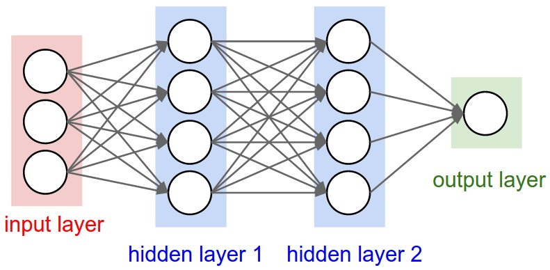
DNN is the composition of miltiple functions. Assuming that $\vec x$ is the input and $\vec y$ is the output, a simple DNN can be written as:

$\vec y=h_n(h_{n-1}(…h_1(\vec x)…))$,

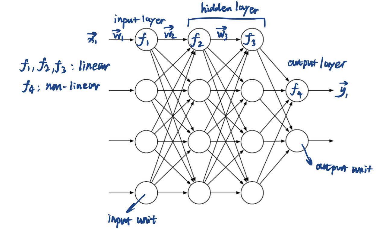
Where $h$ are different functions. These functions can be linear or non-linear. For linear functions, $h_n=w_n h_{n-1}+b_n$, $w_n$ is weight and $b_n$ is bias. For non-linear functions, $h_n=f_n(h_{n-1})$. The $f_n$ here is called as activation function, such as sigmoid function or relu function. The purpose of setting activation function is to make the nerual network more like the human nerual system.

If all the functions are differentiable, we can use chain rule to back propagate the gradient of $\vec y$. Now we have some tools such as Tensorflow or Pytorch to help us compute the gradient automatically. Typically we need a loss function to fit the parameters.

In DNN (as well as CNN) we update weights and biases to get the desired output. In deep Q-learning, the outputs are always some scalers, in other words, Q-value.

Figure 1 shows the structure of a nerual network that is relatively complex. The important components of one of the routes is marked. Figure 2 shows the detailed structure of a node.

Benefits

• Uses distributed representations instead of local representations
• Universal function approximator
• Can potentially need exponentially less nodes/parameters to represent the same function
• Can learn the parameters using SGD

Convolutional Nerual Network (CNN)

CNN is widely used in computer vision. If you want to make decisions using pictures, CNN is very useful for visual input.

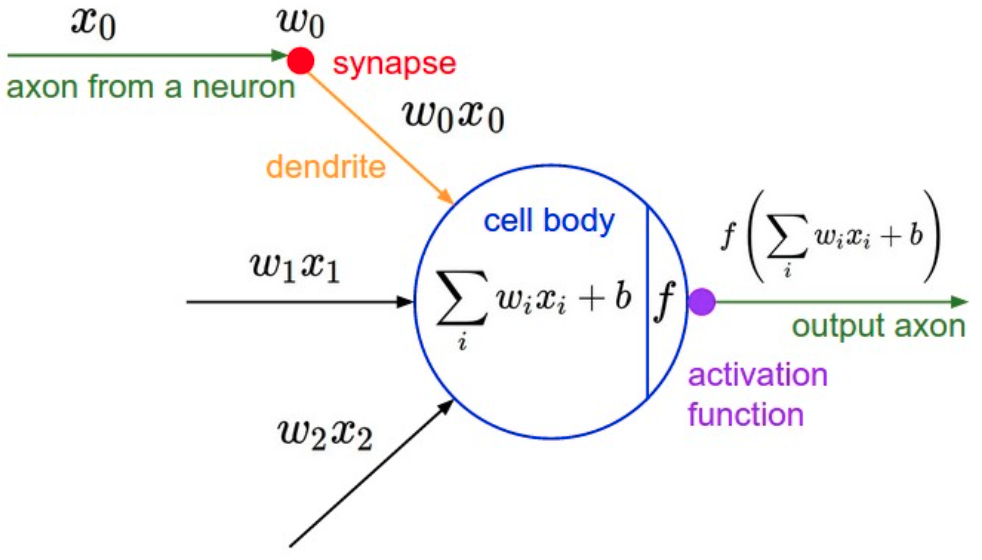
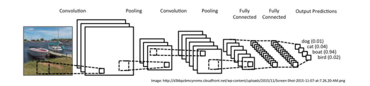
Images have structure, they have local structure and correlation. They have distictive features in space and frequency domain. CNN can extract these features and give the output. Figure 3 shows the basic process as well as some features of CNN.

Now I am going to give you a brief introduction of how a CNN works.

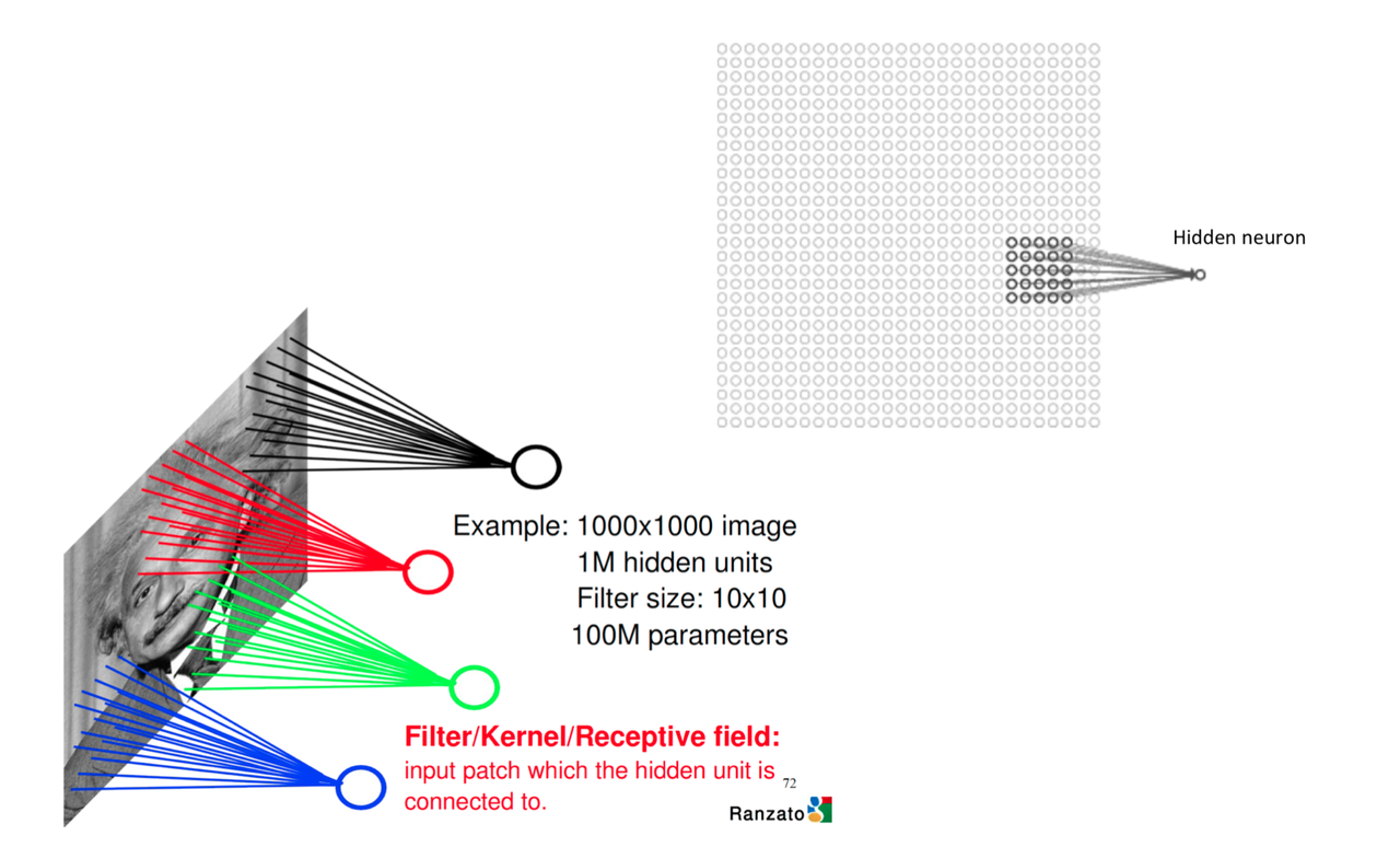
Receptive Field

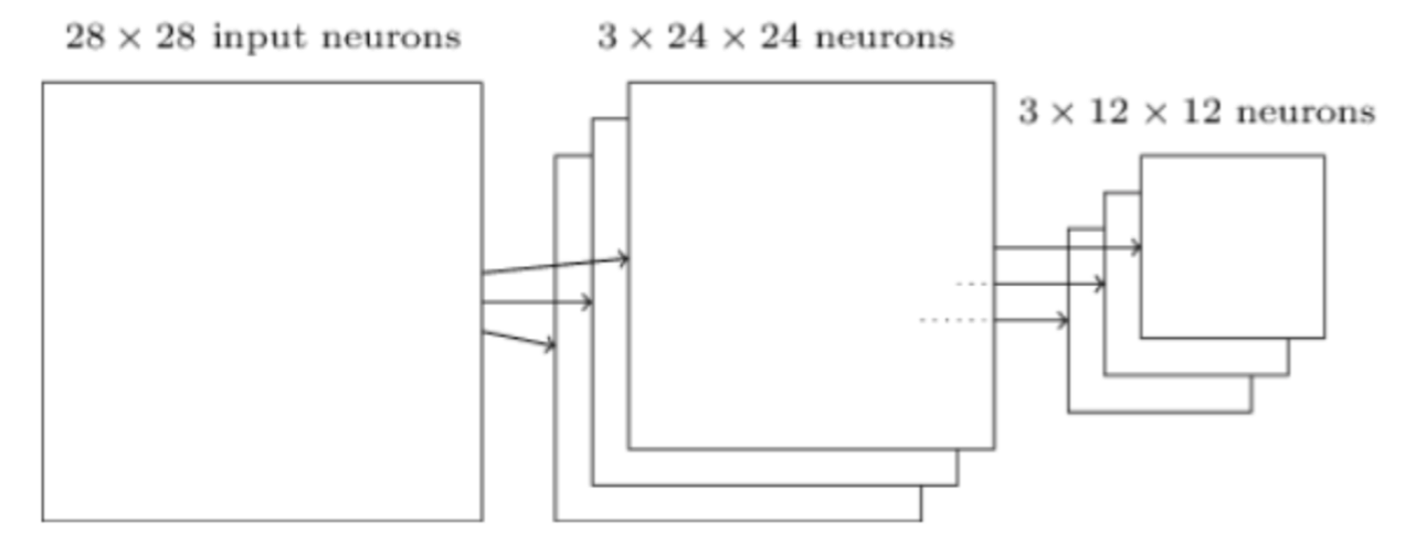
First, we need to randomly choose a part of the image as the input of a hidden unit. That part chosen from the image is called as filter/kernel/receptive field (we will call it filter after that). The range of the filter is called filter size. In the example showned in Figure 3, the filter size is $5\times 5$. One CNN will have many filters and they form what we called input batch. Input batch is connected to the hidden units.

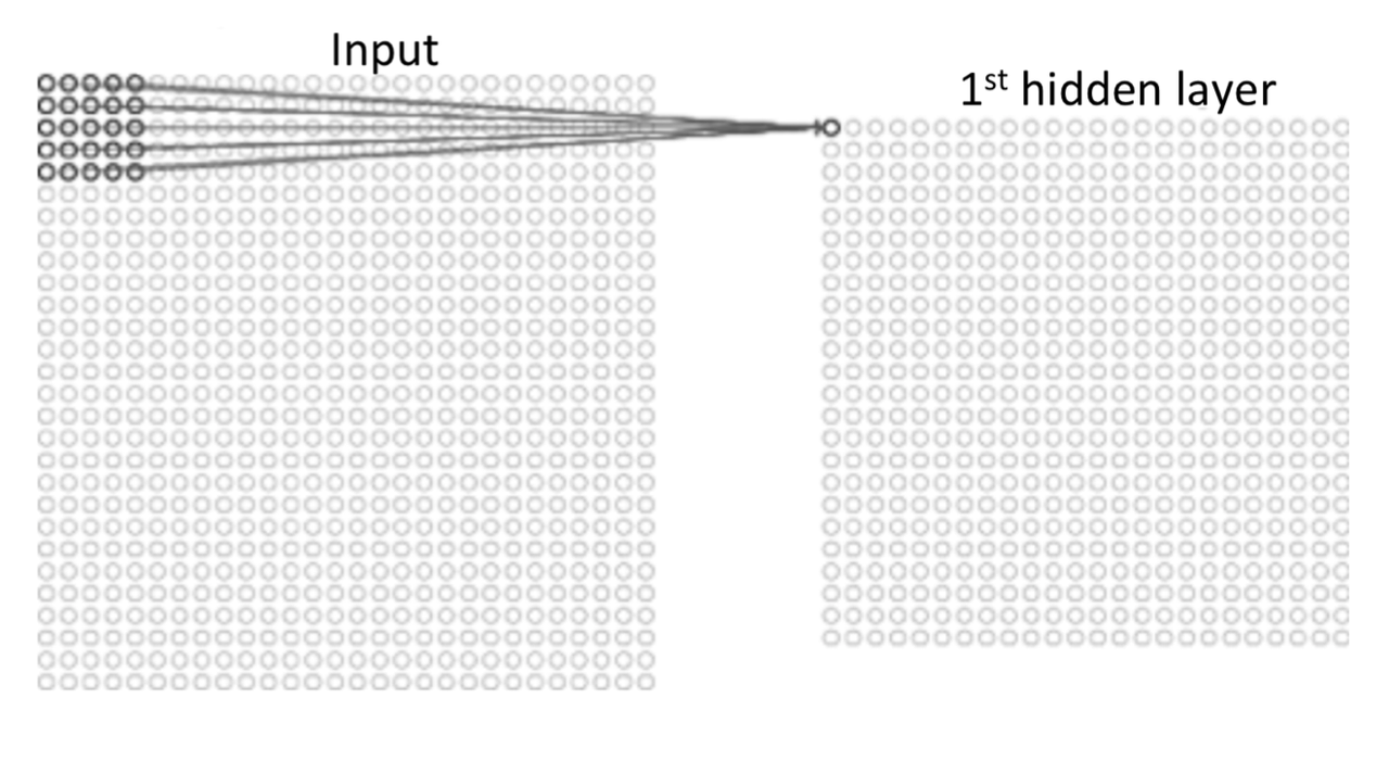
Stride

Now we want the filter to scan all over the image. We can slide the $5\times5$ filter over all the input pixels. If the filter move 1 pixel each time it slides, we define that the stride length is 1. Of course we can use other stride lengths. Assume the input is $28\times28$, than we need to move $24\times24$ times and we will have a $24\times24$ first hidden-layer. For a filter, it will have 25 weights.

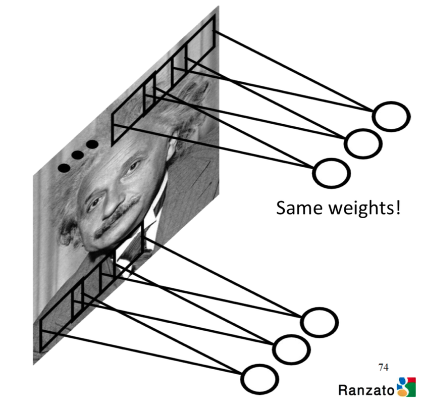
Shared Weights and Feature Map

For a same feature in the image, we want the algorithm able to recognize it no matter it is showned in any part of it (left side, right side, etc.) or in any direction (vertical, horizontal, etc.). Thus, no matter where the filter moves, we want its weights are always the same. In this example, for the whole CNN we will have 25 weights totally. This feature is called shared weights.

The map from the input layer to the hidden layer is therefore a feature map: all nodes detect the same feature in different parts. The feature map is defined by the shared weights and bias and it is the result of the application of a convolutional filter.

Convolutional Layers

Feature map is the output of convolutional layer. Figure 7 and Figure 8 gives you a visualized example of how it works.

In Figure 8, the green matrix is a image (input) while the yellow matrix in it is a $3\times3$ filter. The red numbers in the filter are weights. The pink matrix at the right is a feature map derives from the left. The value of each unit in feature map is the sum of the value of each unit in the filter times its weight.

Pooling Layers

Pooling layers are usually used immediately after convolutional layers. They compress the information in the output from the convolutional layers. A pooling layer takes each feature map output form convolutional layer and prepares a condensed feature map.

ReLU Layers

ReLU is the abbrivation of rectified linear unit. It is constructed by non-linear functions (activation functions). It increases the nonlinear properties of the overall network without affecting the filters of the convolution layer.

Fully Connected Layers

The process we have talked about is designed to catch the features of the image. After we have done this, we are going to do regression. This work is done by fully connected layers. They can do regression and output some scalers (Q-value in deep Q learning domain).

We now have a rough idea towards CNN. If you want know more about it, you can go to this website.

Deep Q-Learning

Our target is to approximate $\hat q(s,a,\vec w)$ by using a deep neural network and learn neural network parameters $\vec w$. I will give you an example first and then talk about algorithms.

DQN in Atari

Atari is a video game. Researchers tried to apply DQN to train the computer to play this game. The architecture of the DQN they designed is shown in Figure 11.

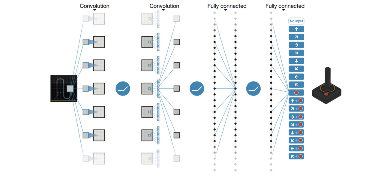
The input to the network consists of an $84\times84\times4$ preprocessed image, followed by three convolutional layers and two fully connected layers with a single output for each valid action. Each hidden layer is followed by a rectifier nonlinearity (ReLU). The network outputs a vector containing Q-values fro each valid action. The reward is change in score for that step.

Preprocessing Raw Pixels

The raw Atari frames are of size $260\times260\times3$, where the last dimension is corresponding to the RGB channels. The preprocessing step aims at reducing the imput dimensionality and dealing with some artifacts of game emulator. The process can be summarized as follows:

• Single frame coding: the maximum value of each pixel color value over the frame being encoded and the previous frame is returned. In other words, we return a pixel-wise max-pooling of the 2 consecutive raw pixel frames.
• Dimensionality reduction: extract the luminance channel, from the encoded RGB frame and rescale it to $84\times84\times1$.

The above preprocessing is applied to the 4 most recent raw RGB frames and the encoded frames are stacked together to produce the input ($84\times84\times4$) to the Q-network.

Training Algorithm for DQN

Essentially, the Q-network is learned by minimizing the following mean squarred error:

$J(\vec w)=\Bbb E_{(s_t,a_t,r_t,s_{t+1})}[(y_t^{DQN}-\hat q(s_t,a_t,\vec w))^2]$,

where $y_t^{DQN}$ is the one-step ahead learning target:

$y_t^{DQN}=r_t+\gamma\tt max_{a’}\mit \hat q(s_{t+1},a’,\vec w^-)$,

where $\vec w^-$ represents the parameters of the target network (belong to CNN, the desire true value) and the parameters $\vec w$ of the online network (belong to function approximator) are updated by sampling gradients from minibatches of past transition tuples $(s_t,a_t,r_t,s_{t+1})$. Notice that when we refer to target network/targets, things are related to the so-called true values provided from Q-network (CNN). And when we refer to online network, things are related to the Q-learning process.

In the last article, we talked about Q-learning with value function approximation. But Q-learning with VFA can diverge. DQN introduces two major changes in order to avoid divergence, which are experience replay and a separate target network.

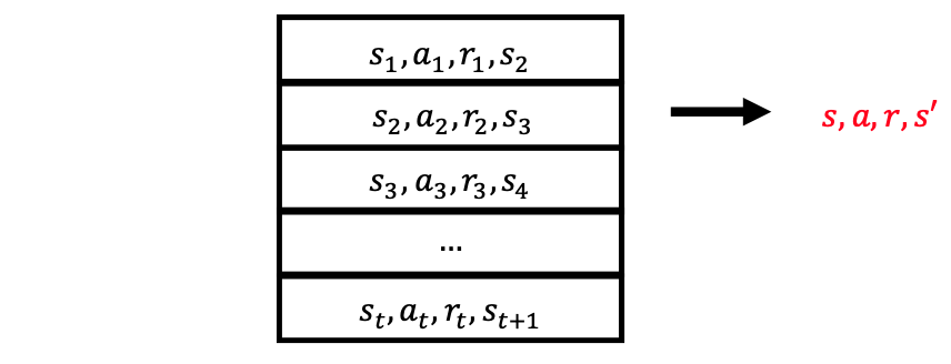
Experience Replay

The agent’s experiences (or transitions) at each time step $e_t=(s_t,a_t,r_t,s_{t+1})$ are stored in a fixed-sized dataset (or replay buffer) $D_t={e_1,…,e_t}$. Figure 12 shows how a replay buffer looks like.

To perform experience replay, we need to repeat the following:

• $(s,a,r,s’)$~$D$: sample an experience tuple form the dataset
• Compute the target value for the sampled $s$: $y_t^{DQN}=r_t+\gamma\tt max_{a’}\mit \hat q(s_{t+1},a’,\vec w^-)$
• Use SGD to update the network weights: $\Delta\vec w=\alpha[r+\gamma\tt max_{a’}\mit\hat q^\pi(s’,a,\vec w^-)-\hat q(s,a,\vec w)]\vec x(s,a)$

Target Network

To further improve the stability of learning and deal with non-stationary learning targets, a separate target network is used for generating the targets $y_j$ in the Q-learning update. More specifically, after every $C$ steps the target network $\hat q(s,a,\vec w^-)$ is updated by copying the parameters’ values $(\vec w^-=\vec w)$ from the online network $\hat q(s,a,\vec w)$, and the target network remains unchanged and generates targets $y_j$ for the following $C$ updates.

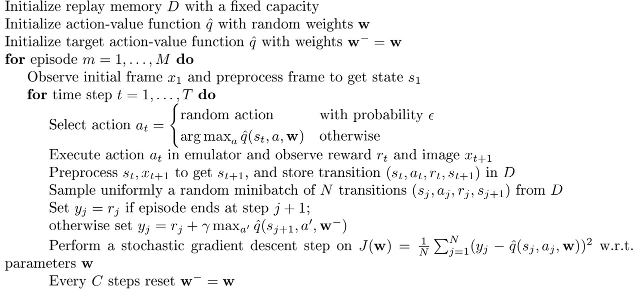
Summary of DQN and Algorithm

• DQN uses experience replay and fixed Q-tragets
• Store transition $(s_t,a_t,r_t,s_{t+1})$ in replay buffer $D$
• Sample minibatch of transitions $(s,a,r,s’)$ from $D$
• Compute Q-learning target with respect to old, fixed parameters $\vec w^-$
• Optimizes MSE between Q-network and Q-learning targets
• Uses stochastic gradient descent

The algorithm of DQN is shown below:

Double Deep Q-Network (DDQN)

After the successful application of DQN to Atari, people become very interested in it and developed many other improvements, while DDQN and Dueling DQN are two very popular algorithms among them. Let’s talk about DDQN first.

Recall in Double Q-learning, in order to eliminate maximization bias, two Q-functions are maintained and learned by randomly assigning transitions to update one of two functions, resulting two different sets of parameters, denote here as $w$ and $w’$. This idea can also be extented to deep Q-learning.

The target network in DQN architecture provides a natural candidate for the second Q-function, without introducing additional networks. Similarly, the greedy action is generated accroding to the online network with parameters $w$, but its value is estimated by the target network with parameters $w^-$. The resulting algorithm is reffered as DDQN, which just slightly change the way $y_t$ updates:

$y_t^{DDQN}=r_t+\gamma\hat q(s_{t+1},\tt argmax_{a’}\mit\hat q(s_{t+1},a’,\vec w),\vec w^-)$.

Dueling DQN

Before we delve into dueling architecture, let’s first introduce an important quantity, the advantage function, which relates the value and Q-functions (assume following a policy $\pi$):

$A^\pi(s,a)=Q^\pi(s,a)-V^\pi(s)$.

Intuitively, the advantage function sbstracts the value of the state from the Q funciton to get a relative measure of the importance of each action.

DQN approximates the Q-function by decoupling the value function and the advantage function. Figure 13 illustrates the dueling network architecture and the DQN for comparison.

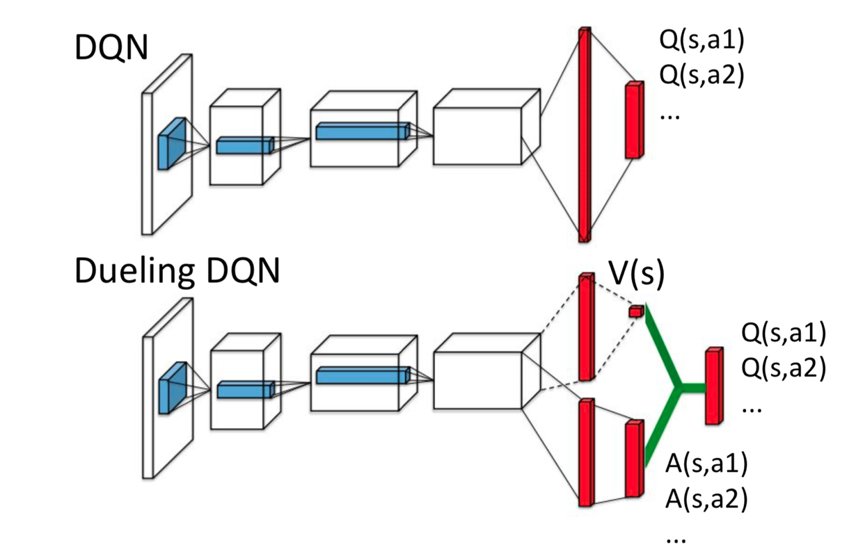
The different between dueling network and DQN is that, the dueling network uses two streams of fully connected layers. One stream is used to provide value function estimate given a state, while the other stream is for estimating advantage function for each valid action. Finally, the two streams are comined in a way to produce and approximate the Q-function.

Why these two separated streams are designed? First, for many states, it is unnecessary to estimate the value of each possible action choice. Second, features required to determine the value function may be different than those used to accurately estimate action benefits.

Let’s denote the scalar output value function from one stream of fully-connected layers as $\hat v(s,\vec w,\vec w_v)$, and denote the vector output advantage function from the other stream as $A(s,a,\vec w,\vec w_A)$. We use $\vec w$ here to denote the shared parameters in the convolutional layers, and use $\vec w_v$ and $\vec w_A$ to represent parameters in the two different streams of fully-connected layers. According to the definition of advantage function, we have:

$\hat q(s,a,\vec w,\vec w_v,\vec w_A)=\hat v(s,\vec w,\vec w_v)+A(s,a,\vec w,\vec w_A)$.

However, the expression above is unidentifiable, which means we can not recover $\hat v$ and $A$ form a given $\hat q$. This unidentifiable issue is mirrored by poor performance in practice.

To make Q-function identifiable, we can force the advantage function to have zero estimate at the chosen action. Then, we have:

$\hat q(s,a,\vec w,\vec w_v,\vec w_A)=\hat v(s,\vec w,\vec w_v)+(A(s,a,\vec w,\vec w_A)-\tt max_{a’\in A}\mit A(s,a’,\vec w,\vec w_A))$.

Or we can just use mean as baseline:

$\hat q(s,a,\vec w,\vec w_v,\vec w_A)=\hat v(s,\vec w,\vec w_v)+(A(s,a,\vec w,\vec w_A)-{1\over|A|}\sum_{a’}A(s,a’,\vec w,\vec w_A))$.