Summary of Reinforcement Learning 5

Introduction

So far we have presented value function by a lookup table (vector or matrix). However, this approach might not generalize or sufficient well to problems with very large state and/or action spaces in reality.

A popular approach to address this problem via function approximation: $v_\pi(s)\approx \hat v(s,\vec w)$ or $q_\pi(s,a)\approx\hat q(s,a,\vec w)$. Here $\vec w$ is usually referred to as the parameter or weights of our function approximator. Our target is to output a reasonable value function (it can also be called as update target in this domain) by calculating the proper $\vec w$ with the input $s$ or $(s,a)$.

In this set of article, we will explore two popular classes of differentiable function approximators: Linear feature representations and Nerual networks. We will only focus on linear feature representations in this article.

Linear Feature Representations

Gradient Descent

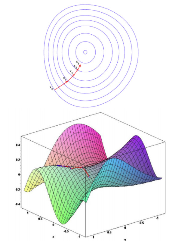
The rough definition of gradient is that, for a function that has several variables, gradient (a vector) at a spot $x_0$ tells us the direction of the steepest increase in the objective function at $x_0$. Suppose that $J(\vec w)$ is an arbitrary function and vector $\vec w$ is its parameter, the gradient of it at some initial spot $\vec w$ is:

$\nabla_\vec wJ(\vec w)=[{\partial J(\vec w)\over\partial w_1}{\partial J(\vec w)\over\partial w_2}…{\partial J(\vec w)\over\partial w_n}]$.

In oreder to minimize our objective function, we take a step along the negative direction of the gradient vector and arrive at $\vec w’$, mathematically written as:

$\Delta\vec w=-{1\over 2}\alpha \nabla_\vec wJ(\vec w)$, $\vec w’=\vec w+\Delta \vec w$ ($\alpha$ is update step).

By using this way for many times we can reach the point that our objective function is minimize (local optima).

Figure 1 is the visualization of gradient descent.

####Stochastic Gradient Descent (SGD)

In linear function representations, we use a feature vector to represent a state:

$\vec x(s)=[x_1(s)\ x_2(s)\ …\ x_n(s)]$.

We than approximate our value functions using a linear combination of features:

$\hat v(s,\vec w)=\vec x(s)\vec w=\sum_{j=1}^nx_j(s)w_j$.

Our goal is to find the $\vec w$ that minimizes the loss between a true value function $v_\pi(s)$ and its approximation $\hat v(s,\vec w)$. So now we define the objective function (also known as the loss function) to be:

$J(\vec w)=\Bbb E[(v_\pi(s)-\hat v(s,\vec w))^2]$.

Then we can use gradient descent to calculate $\vec w’$ ($w$ at next time step):

$\vec w’=\vec w-{1\over2}\alpha\nabla_\vec w[(v_\pi(s)-\hat v(s,\vec w))^2]$

​ $=\vec w+\alpha[v_\pi(s)-\hat v(s,\vec w)]\nabla_\vec w\hat v(s,\vec w)$.

However, it is impossible for us to know the true value of $v_\pi(s)$ in real world. So we will then talk about how to do value function approximation without a model, or, in other words, find something to replace the true value to make this idea practicable.

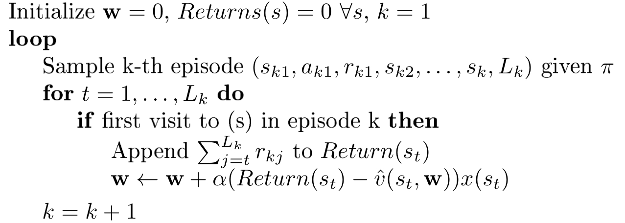
Monte Carlo with Linear Value Function Approximation (VFA)

As we know, the return $G$ is an unbiased sample of $v_\pi(s)$ with some noise. So if we substituted $G$ for $v_\pi(s)$, we have:

$\vec w’=\vec w+\alpha[G-\hat v(s,\vec w)]\nabla_\vec w\hat v(s,\vec w)$

​ $=\vec w+\alpha[G-\hat v(s,\vec w)]\vec x(s)$.

Tha algorithm of Monte Carlo linear value function approximation is shown below:

.

This algorithm can also be modified into a every-visit type. Once we have $\vec w’$ we can calculate the approximation of the value function $\hat v(s,\vec w)$ by $\vec x(s)^T\vec w’$.

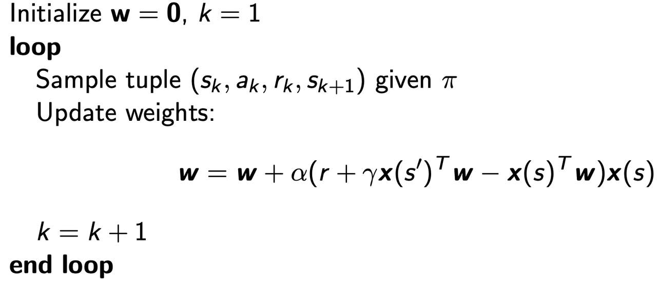
Temporal Difference with Linear VFA

In TD learning we use $V^\pi(s_t)=V^\pi(s_t)+\alpha(r_t+\gamma V^\pi(s_{t+1})-V^\pi(s_t))$ to update $V^\pi$. To apply this method to VFA, we can rewrite the expression of $\vec w$ as:

$\vec w’=\vec w+\alpha[r+\gamma \hat v^\pi(s’,\vec w)-\hat v(s,\vec w)]\nabla_\vec w\hat v(s,\vec w)$

​ $=\vec w+\alpha[r+\gamma \hat v^\pi(s’,\vec w)-\hat v(s,\vec w)]\vec x(s)$.

The algorithm of TD(0) with linear VFA is shown below:

.

The two algorithm we introduced above can both converge to the weights $\vec w$ with different minimum mean squared error (MSE). Among them the MSE of TD method is slightly greater than the MC one, but it is good engouh.

Control Using VFA

Similar to VFAs, we can also use function approximator for action-values and we let $q_\pi(s,a)\approx\hat q(s,a,\vec w)$. In this part we will use VFA to approximate policy evaluation and than perform $\epsilon$-greedy policy improvement. However, this process can be unstable because it involes the intersection of function approximation, bootstrapping, and off-policy learning. These three things are called as the dadely triad, which may make the result fail to converge or converge to something bad. Now I will quickly pass this part using the basic concept we have mentioned before.

First we define our objective function $J(\vec w)$ as:

$J(\vec w)=\Bbb E[(q_\pi(s,a)-\hat q^\pi(s,a,\vec w))^2]$.

Then we define the state-action value feature vector:

$\vec x(s,a)=[x_1(s,a)\ x_2(s,a)\ …\ x_n(s,a)]$,

and represent state-action value as linear combinations of features:

$\hat q(s,a,\vec w)=\vec x(s,a)\vec w$.

Compute the gradient:

$-{1\over 2}\nabla_\vec wJ(\vec w)=\Bbb E_\pi[(q_\pi(s,a)-\hat q^\pi(s,a,\vec w))\nabla_\vec w\hat q^\pi(s,a,\vec w)]$

​ $=(q_\pi(s,a)-\hat q^\pi(s,a,\vec w))\vec x(s,a)$.

Compute an update step using gradient descent:

$\Delta\vec w=-{1\over 2}\alpha\nabla_\vec wJ(\vec w)$

​ $=\alpha(q_\pi(s,a)-\hat q_\pi(s,a,\vec w))\vec x(s,a)$.

Take a step towards the local minimum:

$\vec w’=\vec w+ \Delta\vec w$.

Just like what we have said before, we cannot get the true value of $q_\pi(s,a)$ so we gonna use other values to replace it and the difference between those methods is the difference of the value we choose.

For Monte Carlo methods, we use return $G$, and the update becomes:

$\Delta\vec w=\alpha(G-\hat q_\pi(s,a,\vec w))\vec x(s,a)$.

For SARSA we have:

$\Delta\vec w=\alpha[r+\gamma \hat q^\pi(s’,a,\vec w)-\hat q(s,a,\vec w)]\vec x(s,a)$.

And for Q-learning:

$\Delta\vec w=\alpha[r+\gamma\tt max_{a’}\mit\hat q^\pi(s’,a,\vec w)-\hat q(s,a,\vec w)]\vec x(s,a)$.

Notice that because of the value function approximations, which can be expansions, converge is not guaranteed. The table below gives the summary of convergence of control methods with VFA and (Yes) means the result chatters around near-optimal value function.

Algorithm	Tabular	Linear VFA	Nonlinear VFA
MC Control	Yes	(Yes)	No
SARSA	Yes	(Yes)	No
Q-learning	Yes	No	No

In the next article we will talk about deep reinforcement learning using nerual networks.