Summary of Reinforcement Learning 4

Introduction

In this article we will discuss model-free control where we learn good policies under the same constrains (only interactions, no knowledge of reward structure or transition probabilities). In actual world, many problems can be modeled into a MDP and model-free control is important for some problems in two types of domains:

• MDP model is unknown but we can sample the trajectories from the MDP
• MDP model is known but computing the value function is really really hard due to the size of the domain

There are two types of policy learning under model-free control domain, which are on-policy learning and off-policy learning.

• On-policy learning: base on direct experience and learn to estimate and evaluate a policy from experience obtained from following that policy
• Off-policy learning: learn to estimate and evaluate a policy using experience gathered from following a different policy

Generalized Policy Iteration

In Summarize of Reinforcement Learning 2 we have learned the algorithm of policy iteration, which is:

(1) while True do

(2) $V^\pi$ = Policy evaluation $(M,\pi,\epsilon)$ ($\pi$ is initialized randomly here)

(3) $\pi_{i+1}=\tt argmax\ \mit Q_{\pi i}(s,a)=\tt argmax\mit \ [R(s,a)+\gamma\sum_{s’\in S} P(s’|s,a)V^{\pi i}(s’)]$

(4) if $\pi^*(s)=\pi(s)$ then

(5) break

(6) else

(7) $\pi$ = $\pi^*$

(8) $V^*$ = $V^\pi$ .

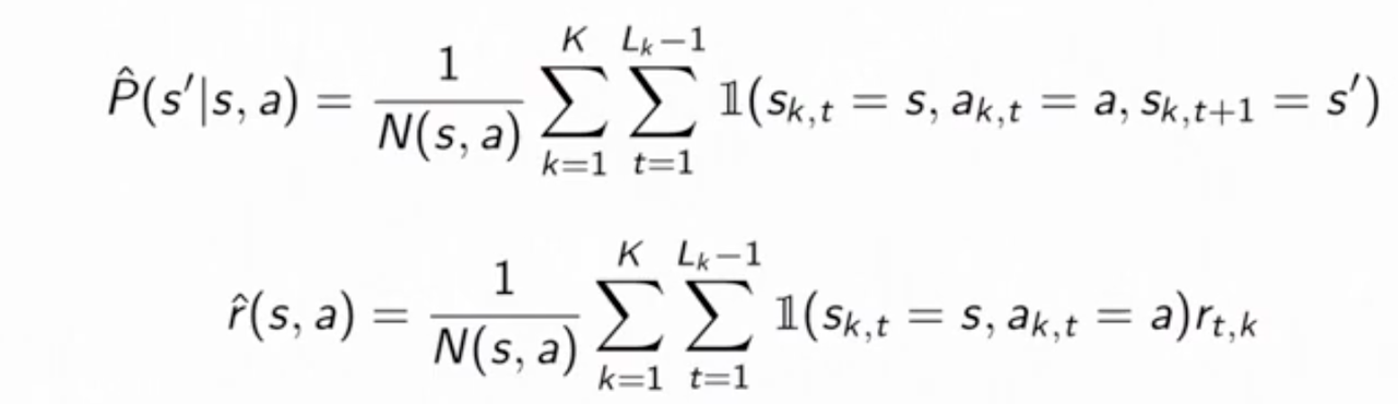
In order to make this algorithm model-free, we can do the policy evaluation (line 2) using the methods we mentioned in the last article. Because we are talking about control, so we use state-action value function $Q^\pi(s,a)$ to substitute $V^\pi$ in line 2, in a Monte Carlo way. The algorithum of MC for policy Q evaluation is written below:

Initialize $N(s,a)=0,\ G(s,a)=0,\ Q^\pi(s,a)=0,\ \forall s\in S,\ a\in A$

Using policy $\pi$ to sample an episode $i=s_{i,1},a_{i,1},r_{i,1},…$

while each state, action $(s,a)$ visited in episode $i$ do

​ while first/every time $t$ that the state, action $(s,a)$ is visited in episode $i$ do

​ $N(s,a)=N(s,a)+1$

​ $G(s,a)=G(s,a)+G_{i,t}$

​ $Q^{\pi i}(s,a)=Q^{\pi i}(s,a)/N(s,a)$

return $Q^{\pi i}(s,a)$.

Thereby, accroding to the definition, we can modify the line 3 directly as:

$\pi_{i+1}=\tt argmax\ \mit Q_{\pi i}(s,a)$.

There are a few caveats to this modified algorithm (MC for policy Q evaluation):

• If policy $\pi$ is determiniistic or dosen’t take every action with some positive probability, then we cannot actually compute the argmax in line 3
• The policy evaluation algorithm gives us an estimate of $Q^\pi$, so it is not clear whether (while we want to make sure that) line 3 will monotonically improve the policy like the model-based case.

Importance of Exploration

Please notice the first caveat we just mentioned above, this means, in other words, the policy $\pi$ needs to explore actions, even if they might be suboptimal with respect to our current Q-value estimates. And this is what we have talked about in the first article: the relationship between exploration and exploitation. Here is a simple way to balance them.

$\epsilon$-greedy Policies

This strategy is to take random action with small probability and take the greedy action the rest of the time. Mathematically, an $\epsilon$-greedy policy with respect to the state-action value $Q^\pi(s,a)$ takes the following form:

.

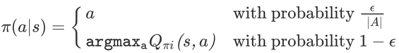It can be summarized as: $\epsilon$-greedy policy selects a random action with probability $\epsilon$ or otherwise follows the greedy policy.

Monotonic $\epsilon $-greedy Policy Improvement

We have already provided a strategy to deal with the first caveat and now we are going to focus on the second one: to prove the monotonic $\epsilon$-greedy policy improvement. And here is the proof.

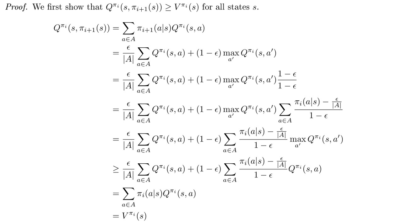
Now we have that $Q^{\pi_i}(s,\pi_{i+1}(s))\ge V^{\pi_i}(s)$ implies $V^{\pi_{i+1}}(s)\ge V^{\pi_i}$ for all states, as desired. Thus, the monotonic $\epsilon $-greedy policy improvement shows us that our policy does in fact improve if we act $\epsilon$-greedy on the current $\epsilon$-greedy policy.

Greedy in the Limit of Infinite Exploration (GLIE)

$\epsilon$-greedy is a naive way to balance exploration and exploitation and we can refine it. The new class of exploration strategies is called Greedy in the Limit of Infinite Exploration (GLIE), which allows us to make convergence guarantees about our algorithms.

A policy is GLIE if it satisfies the following two properties:

• All state-action pairs are visited an infinite number of times: $\lim_{i\rightarrow\infty}N_i(s,a)\rightarrow\infty$
• Behavior policy converges to greedy policy

A simple GLIE strategy is $\epsilon$-greedy policy where $\epsilon$ is decayed to zero with $\epsilon_i={1\over i}$, $i$ is the epsiode number.

Monte Carlo Control

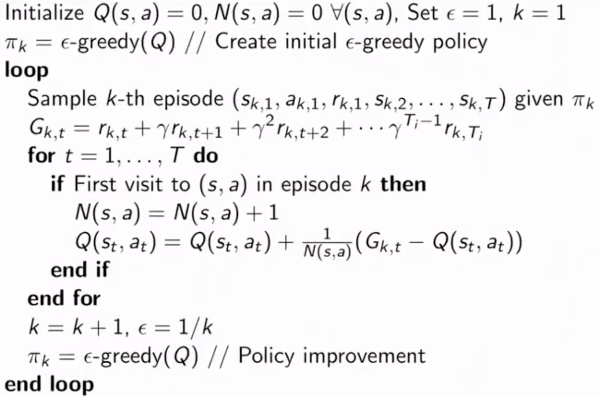
Here is the algorithm of online Monte Carlo control:

.

The algorithm is first-visit online Monte Carlo control precisely and you can modify it to every-visit online Monte control easily.

If $\epsilon$-greedy strategy used in this algorithm is GLIE, then the Q-value derived from the algorithm will converge to the optimal Q-function.

Tempooral Difference Methods for Control

There are two methods of TD-style model-free control: on-policy and off-policy. We first introduce the on-policy method, called SARSA.

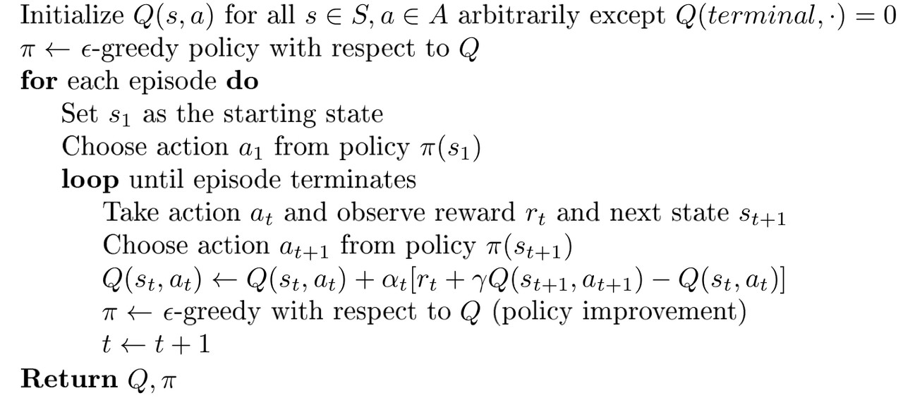
SARSA

Here is the algorithm:

.

SARSA stands for State, Action, Reward, next State, Action taken in next state. Because this algorithm updates the Q-value after it gets the tuple $(s,a,r,s’,a’)$, it is called SARSA. SARSA is an on-policy method because the actions $a$ and $a’$ used in the update equation are both from the policy that is being followed at the time of the update.

SARSA for finite-state and finite-action MDP’s converges to the optimal action-value if the following conditions hold:

• The sequence of policies $\pi$ from is GLIE
• The step-sizes $\alpha_t$ satisfy the Robbins-Munro sequence such that: $\sum^\infty_{t=1}\alpha_t=\infty,\ \sum^\infty_{t=1}\alpha_t^2<\infty$ (although we generally don’t use the step-sizes satisfy this condition in reality).

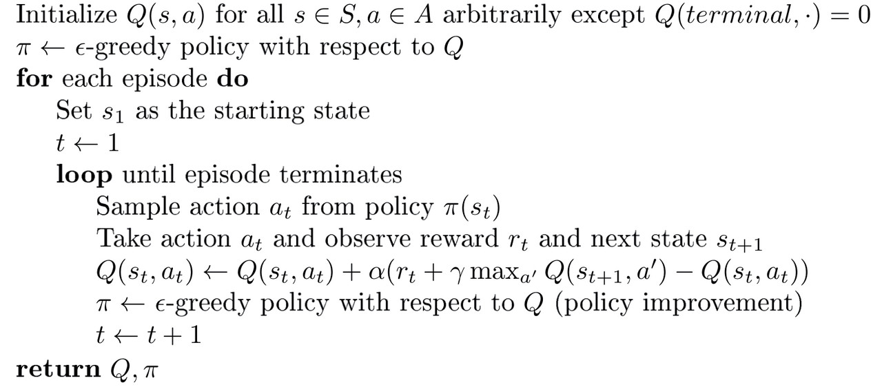
Q-Learning

Here is the algorithm:

.

The biggest different between Q-learning and SARSA is that, Q-learning takes a maximum over the actions at the next state, this action is not necessarily the same same as the one we would derive from the current policy. On the contrary, the agent will choose the action that brings the biggest reward directly and this behavior actually updates the policy because, when we adopt $\epsilon$-greedy we definately introduce Q-value. Q-learning updates the Q-value (policy) after it gets the tuple $(s,a,r,s’)$. And this is why it is called off-policy.

However, in SARSA, as we stated before, the action $a’$ derives from the current policy that has not been updated. The agent may choose a bad action $a’$ randomly following the $\epsilon$-greedy policy and this may lower the Q-value of some state-action pairs after the update. This consequently lead to the result that, SARSA might not figure out the optimal trajectory of the agent but the suboptimal one.

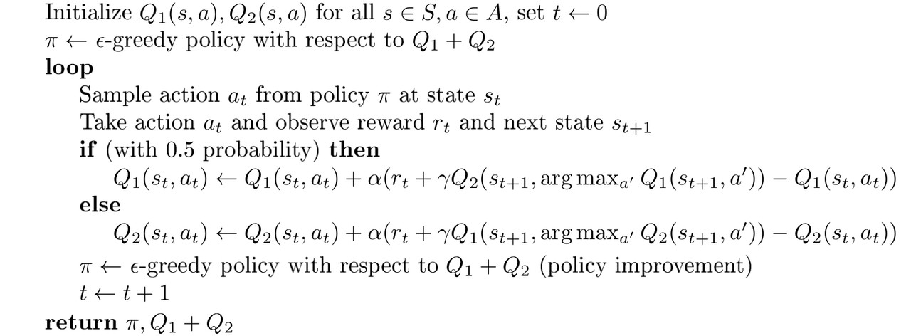
Double Q-Learning

In Q-learning, the state values $V^\pi(s)=\sum_{a\in A}\pi(a|s)Q_\pi(s,a)$ can suffer from maximization bias (bias introduced by the maximization operation) when we have finitely many samples. Our state value estimate is at least as large as the true value of state $s$, so we are systematically overestimating the value of the state. In Q-learning, we can maintain two independent unbiased estimates, $Q_1$ and $Q_2$ and when we use one to select the maximum, we can use the other to get an estimate of the value of this maximum. This is called double Q-learning which is shown below:

.

Double Q-learning can significantly speed up training time by eliminating suboptimal actions more quickly then normal Q-learning.