Summary of Reinforcement Learning 3

Introduction

In the previous article we talked about MP, MRP, MDP and how to find the best policy. All the discussions are based on the fact that we know both the rewards and probabilities for every transition. However, in many cases such information is not readily available to us. Therefore, we are going to discuss model-free algorithms in this article.

Throughout this article, we will assume an infinite horizon as well as stationary rewards, transition probabilities and policies.

First comes the definition of history: the history is the ordered tuple of states, actions and rewards that an agent experiences. The $j$ th history is:

$h_j=(s_{j,1},a_{j,1},r_{j,1},s_{j,2},a_{j,2},r_{j,2},…,s_{j,L_j})$,

where $L_j$ is the length of the interaction (interaction between agent and environment).

In the article Summary of Reinforcement Learning 2 I introduced the iterative solution of value function, which is

$V_t(s)=\Bbb E_\pi[R_{t+1}+\gamma V_\pi (s_{t+1})|s_t=s]$

​ $=R(s)+\gamma \sum P(s’|s)V_{t+1}(s’), \forall t=0,…,H-1,V_H(s)=0$.

This ia a bootstraping process, and we estimate the value of the next state using our current estimate of next state.

Monte Carlo on policy evaluation

In general, we got the Monte Carlo estimate of some quantity by iterations of how that quantity is generated either in real life or via simulation and then averaging over the observed quantities. By the law of large numbers, this average converges to the expectation of the quantity.

In reinforcement learning the quantity we want to estimate is $V^\pi(s)$ and we can get it through three steps:

• Execute a rollout of policy until termination many times
• Record the returns $G_t$ that we observe when starting at state $s$
• Take an average of the values we got for $G_t$ to estimate $V^\pi(s)$.

Figure 1 shows a backup diagram for the Monte Carlo policy evaluation algorithm. And you can find that, unlike what we have talked about in the second article, Monte Carlo on policy evaluation is not a bootstraping process.

How to Evaluate the Good and Bad of an Algorithm?

We use three quntities to evaluate the good and bad of an algorithm.

Consider a statistical model that is parameterized by $\theta$ and that determins a probability distribution over oberserved data $P(x|\theta)$. Then consider a statistic $\hat\theta$ that provides an estimate of $\theta$ and it’s a function of observed data $x$. Then we have these quantities of the estimator:

Bias: $Bias_\theta(\hat\theta)=\Bbb E\rm_{x|\theta}[\hat\theta]-\theta$,

Variance: $Var(\hat\theta)=\Bbb E\rm_{x|\theta}[(\hat\theta-\Bbb E\rm[\hat\theta])^2]$,

Mean squared error (MSE): $MSE(\hat\theta)=Var(\hat\theta)+Bias_\theta(\hat\theta)$.

First-Visit Monte Carlo

Here is the algorithm of First-Visit Monte Carlo:

Initialize $N(s)=0,\ G(s)=0,\ V(s)=0,\ \forall s\in S$

$N(s)$: Increment counter of total first visits

$G(s)$: Increment total return

$V(s)$: Estimate

while each state $s$ visited in episode $i$ do

​ while first time $t$ that the state $s$ is visited in episode $i$ do

​ $N(s)=N(s)+1$

​ $G(s)=G(s)+G_{i,t}$

​ $V(s)=G(s)/N(s)$

return $V(s)$

First-Visit Monte Carlo estimator is an unbised estimator.

Every-Visit Monte Carlo

Here is the algorithm of Every-Visit Monte Carlo:

Initialize $N(s)=0,\ G(s)=0,\ V(s)=0,\ \forall s\in S$

$N(s)$: Increment counter of total first visits

$G(s)$: Increment total return

$V(s)$: Estimate

while each state $s$ visited in episode $i$ do

​ while every time $t$ that the state $s$ is visited in episode $i$ do

​ $N(s)=N(s)+1$

​ $G(s)=G(s)+G_{i,t}$

​ $V(s)=G(s)/N(s)$

return $V(s)$.

Every-Visit Monte Carlo is a bised estimator becaue the varibles are not IID (Independently Identicaly Distribution). But it has a lower variance which is better than First-Visit Monte Carlo.

Increment First-Visit/Every-Visit Monte Carlo

We can replace $V(s)=G(s)/N(s)$ in both two algorithms by

$V(s)=V(s)+{1\over N(s)}(G(s)-V(s))$.

Because

${V(s)(N(s)-1)+G(s)\over N(s)}=V(s)+{1\over N(s)}(G(s)-V(s))$.

Replacing $1\over N(s)$ with $\alpha$ in the upper expression gives us the more general Incremental Monte Carlo on policy evaluation. Setting $\alpha > {1\over N(s)}$ gives higher weight to newer data, which can help learning in non-stationary domains.

Temporal Difference (TD) Learning

TD learning is a new algorithm that combines bootstraping with sampling. It is still model-free, and it will update its value after every observation.

In dynamic programming, the return is witten as $r_t+\gamma V^\pi(s_{t+1})$, where $r_t$ is a sample of the reward at time step $t$ and $V^\pi(s_{t+1})$ is our current estimate of the value at the next state. We can use the upper expression to replace the $G(s)$ in the incremental Monte Carlo update and then we have

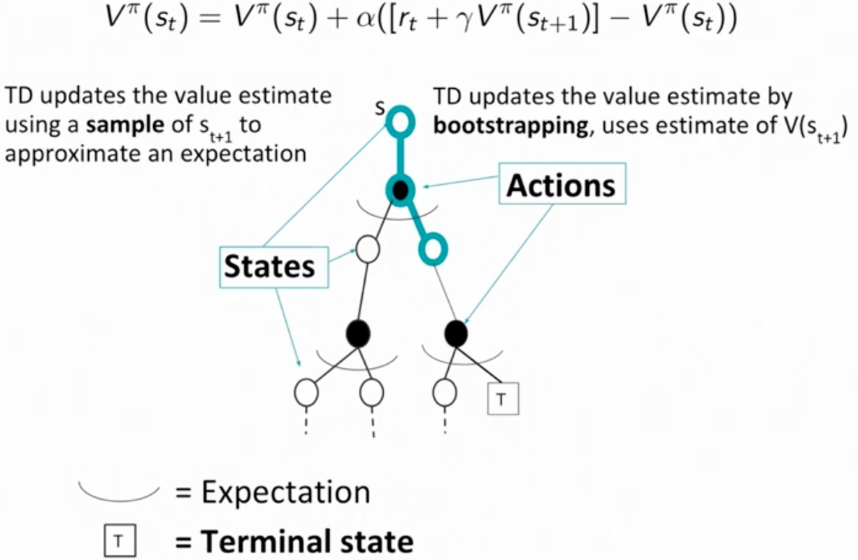
$V^\pi(s_t)=V^\pi(s_t)+\alpha(r_t+\gamma V^\pi(s_{t+1})-V^\pi(s_t))$,

and this is the TD learning update.

In TD learning update, there are two concepts which are TD error and TD target. TD error is written as below:

$\delta_t=r_t+\gamma V^\pi(s_{t+1})-V^\pi(s_t)$.

And here is TD target, which is the sampled reward combined with the bootstrap estimate of the next state value:

$r_t+\gamma V^\pi(s_{t+1})$.

The algorithm of TD learning is shown below.

Initialize $V^\pi(s)=0,\ s\in S$

while True do

​ Sample tuple $(s_t,a_t,r_t,s_{t+1})$

​ $V^\pi(s_t)=V^\pi(s_t)+\alpha(r_t+\gamma V^\pi(s_{t+1})-V^\pi(s_t))$

It is improtance to aware that $V^\pi(s_{t+1})$ is the current value (estimate) of the next state $s_{t+1}$ and you can get the exact state at the following next time step. Only at that time can you know what the exact $s_{t+1}$ is and then use the current (you can also regard it as the previous one because it remains the same value at $s_t$) estimate $V^\pi(s_{t+1})$ to calculate the value of $s_t$. Thus that’s why it is called the combination of Monte Carlo and dynamic programming due to the sampling (to approximate the expectation) and bootstraping process.

In reality, if you set $\alpha$ equals to ${1\over N}$ or a very small value, the algorithm will converge definitely. On the contrary, it will oscilate when $\alpha=1$, which means you just ignore the former estimate.

Figure 2 shows a diagram expressing TD learning.

Summary

Table below gives some fundamental properties of these three algorithms (DP, MC, TD).

Properties	DP	MC	TD
Useble when no models of current domain	No	Yes	Yes
Handles continuing domains (episodes will never terminate)	Yes	No	Yes
Handles Non-Markovian domains	No	Yes	No
Coverges to true value in limit (satisfying some conditions)	Yes	Yes	Yes
Unbised estimate of value	N/A	Yes (First-Visit MC)	No
Variance	N/A	High	Low

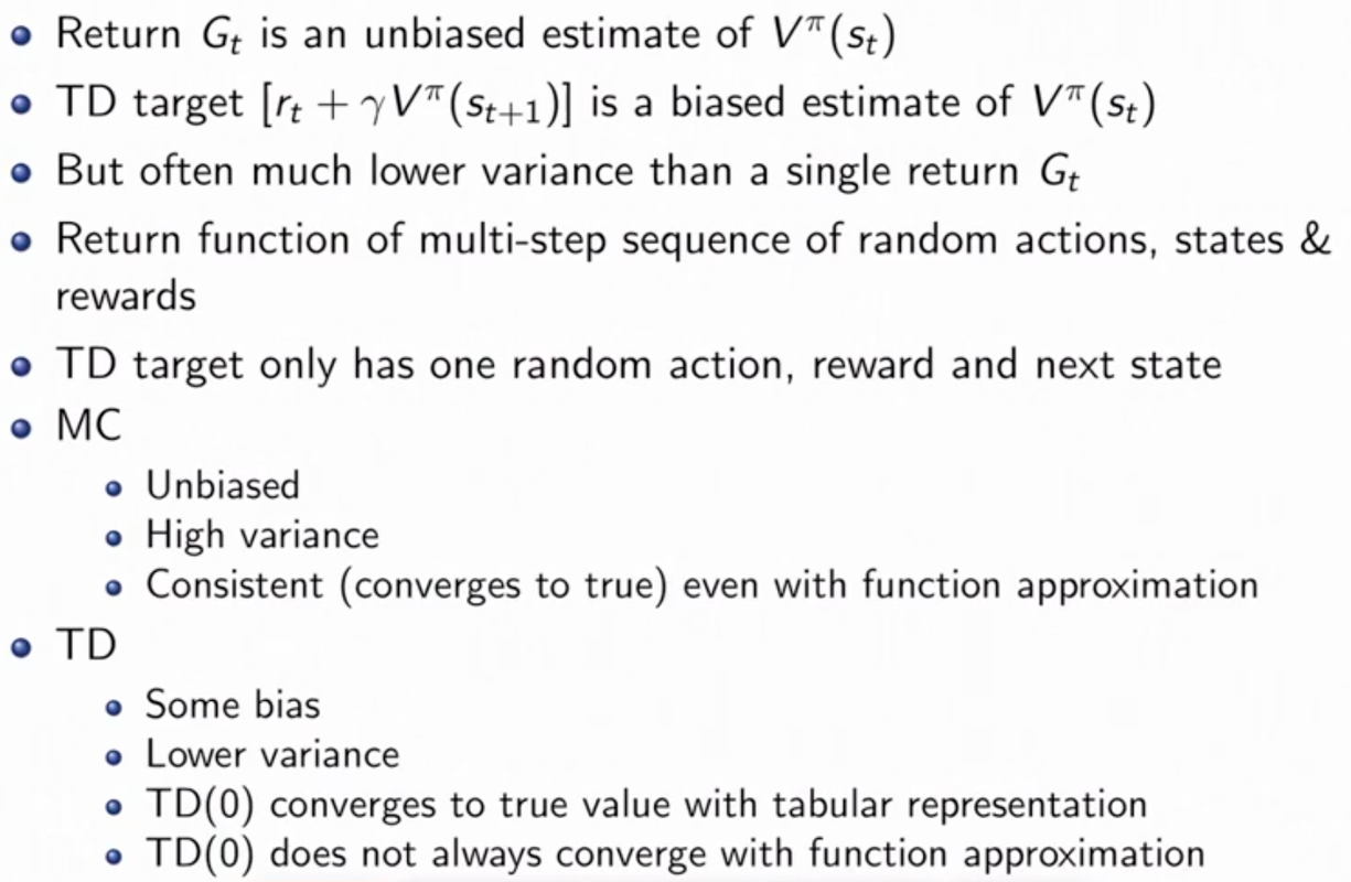
Figure 3 shows some other properties that may help us to choose the algorithm.

Batch Monte Carlo and Temporal Difference

The batch versions of the algorithms is that we have a set of histories that we use to make updates many times and we can use the dataset many times in order to have a better estimate.

In the Monte Carlo batch setting, the calue at each state converges to the value that minimizes the mean squarred error with the observed returns. While in the TD setting, we converge to the value $V^\pi$ that is the value of policy $\pi$ on the maximum likelihood MDP model, where

.

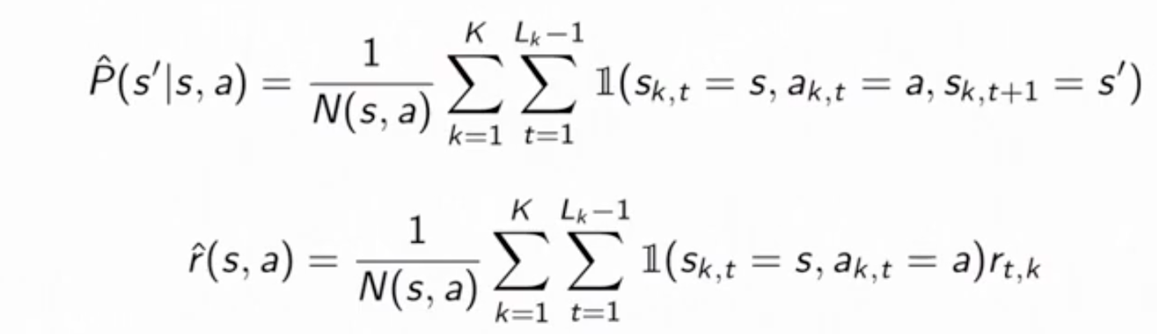The value function derived from the maximum likehood MDP model is known as the certainty equivalence estimate. Using this relationship, we can first compute the maximum likelihoood MDP model using the batch. Then we can compute $V^\pi$ using this model and the model-based policy evaluation methods. This method is highly data efficient but is computationally expensive.