Summary of Reinforcement Learning 2

Markov process (MP)

Markov process is a stochastic process that satisfies the Markov property, which means it is “memoryless” and will not be influenced by the history. MP is sometimes called Markov chain. However, their defination have some slight differences.

We need to make two assumptions before we define the Markov process. The first assumption is that the state of MP is finite, and we have $s_i\in S, i\in1,2,…$ , where $|S|<\infty$. The second assumption is that the transition probabilities are time independent. Transition probabilities are the probability to transform from the current state to a given state, whcih can be written as $P(s_i|s_{i-1}), \forall i=1,2,…$.

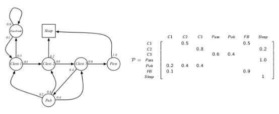
Base on these two assumption, we can define a transition transform matrix:

The size of $\bf P$ is $|S|\times |S|$ and the sum of each row of $\bf P$ equals 1.

Henceforth, we can define a Markov process using a tuple $(S,\bf P)$.

• $S$: A finite state space.
• $\bf P$: A transition probability.

By calculating $S\bf P$ we can get the distribution of the new state.

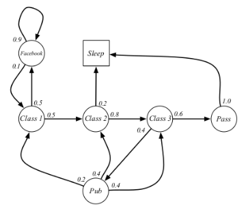
Figure 1 shows a student MP example.

Markov reward process (MRP)

MRP is a MP together with the specification of a reward function $R$ and a discount factor $\gamma$. We can also use a tuple $(S,\bf P,\mit R,\gamma)$ to describe it.

• $S$: A finite state space.
• $\bf P$: A transition probability.
• $R$: A reward function that maps states to rewards (real numbers).
• $\gamma$: Discount factor between 0 and 1.

Here are some explaintions.

Reward function

When we are moving from the current state $s$ to a successor state $s’$, a reward is obtained depending on the current state $s$ (in reality we get the reward at $s’$ ). For a state $s\in S$, we define the expected reward by

$R(s)=\Bbb E[r_t|s_t=s]$.

Here we assume that the reward is time independent. $R$ can be represented as a vector of dimension $|S|$.

Horizon

It is defined as the number of time steps in each episode of the process. An episode is the whole process of a round of training. The horizon can be finite or infinite.

Return

The return $G_t$ is defined as the discounted sum of rewards starting at time $t$ up to the horizon H. We can calculate the return using

$G_t=\sum^{H-1}_{i=t}\gamma^{i-t}r_i$.

State value function

The state value function $V_t(s)$ is defined as the expected return starting from state $s$ and time $t$ and is given by the following expression

$V_t(s)=\Bbb E[G_t|s_t=s]$.

If the episode is determined, then the $G_t$ as well as $V_t(s)$ will remain unchanged. However, because every episode is a random process, the return and state value function will be different in different episodes.

Discount factor

We design the discount factor for many reasons. The best reason among them I think is that, people always pay more attention to the immediate reward rather than the long-term reward. If we set $\gamma <1$, the agent will behave like a human more. We should notice that when $\gamma=0$, we just foucs on the immediate reward. When $\gamma=1$, we put as much importance on future rewards as compared the present.

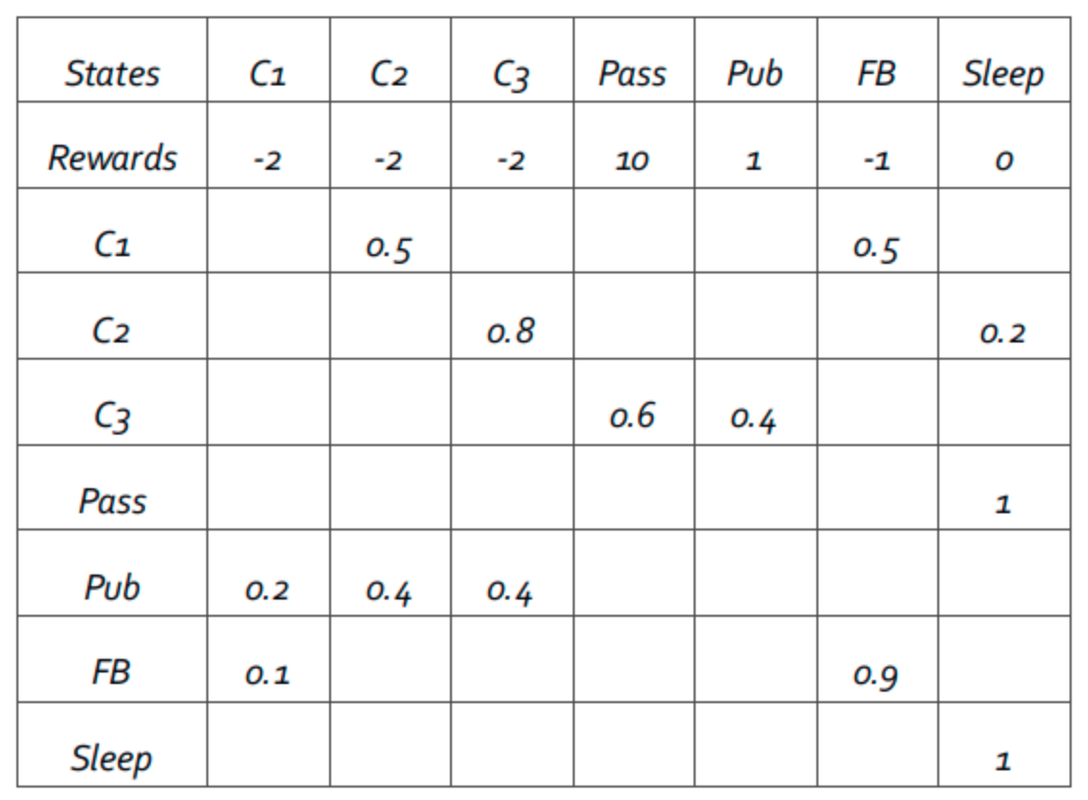
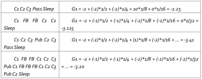
Figure 2 and 3 shows an example of how to calculate the return.

It is significant to find out a value function while many problems of RL is how to get a value function essentially.

Computing the value function

We have three ways to compute the value function.

• Simulation. Through simulation, we can get the value function by averaing many returns of episodes.

• Analytic solution. We have defined the state value function

  $V_t(s)=\Bbb E[G_t|s_t=s]$.

  Then, make a little transformation, see Figure 4 in detail.

  

  Then, we have

  $V(s)=R(s)+\gamma \sum P(s’|s)V(s’)$,

  $V=R+\gamma\bf P\mit V$.

  Therefore we have

  $V=(1-\gamma \bf P\rm )\mit^{-1}R$.

  If $0<\gamma<1$, then $(1-\gamma \bf P\rm)$ is always invertible. However, the computational cost of the analytical method is $O(|S|^3)$, hence it is only suitable for the cases where the $|S|$ is not very large.

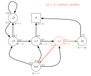
  Notice that $s’$ includes all the possible successor states. Here is an example in Figure 5. This example shows that how to calculate the value of the state represented by the red circle.

  

• Iterative solution.

  $V_t(s)=R(s)+\gamma \sum P(s’|s)V_{t+1}(s’), \forall t=0,…,H-1,V_H(s)=0$.

  We can iterate it again and again and use $|V_t-V_{t-1}|<\epsilon$ ($\epsilon$ is tolerance) to jduge the convergence of the algorithm.

Markov decision process (MDP)

MDP is MRP with the specification of a set of actions $A$. We can use a tuple $(S,A,\bf P,\mit R,\gamma)$ to describe it.

• $S$: A finite state space.
• $A$: A finite set of actions which are available from each state $s$.
• $\bf P$: A transition probability.
• $R$: A reward function that maps states to rewards (real numbers).
• $\gamma$: Discount factor between 0 and 1.

Here are some explanations.

Notifications

• Both $S$ and $A$ are finite.

• In MDP, the transition probabilities at time $t$ are a function of the successor state $s_{t+1}$ along with both the current state $s_t$ and the action $a_t$, written as

  $P(s_{t+1}|s_t,a_t)$.

• In MDP, the reward $r_t$ at time $t$ depends on both $s_t$ and $a_t$, written as

  $R(s,a)=\Bbb E[r_t|s_t=s,a_t=a]$.

• Expect for the value functions and what we have mentioned in this section, other notions are exactly the same as MRP.

Policy

Before we mention the state value function, we need to talk about the policy for the MDP first.

A policy specifies what action to take in each state, which is actually a probability distribution over actions given the current state. The policy may be varying with time, especially when the horizon is finite. A policy can be written as

$\pi(a|s)=P(a_t=a|s_t=s)$.

If given a MDP and a $\pi$, the process of reward satisfies the following two relationships:

• $P^\pi(s’|s)=\sum_{a\in A}\pi(a|s) P(s’|s,a)$

  When we have a policy $\pi$, the probability of the state transforms from $s$ to $s’$ equals to the sum of a series probabilities. These probabilities are the production of the probability to execute a specific action $a$ under the state $s$ and the probability of the state transforms from $s$ to $s’$ when executing an action $a$.

• $R^\pi(s)=\sum_{a\in A}\pi(a|s)R(s,a)$

  When we have a policy $\pi$, the reward of the state $s$ is the sum of the product of he probability to execute a specific action $a$ under the state $s$ and all rewards that the action $a$ can get under the state $s$.

Value functions in MDP (Bellman expectation equations)

Given a policy $\pi$ can define two quantities: the state value function and the state-action value function. These two value functions are both Bellman expectation equations.

• State value function: The state value function $V^\pi_t(s)$ for a state $s\in S$ is defined as the expected return starting from the state $s_t=s$ at time $t$ and the following policy $\pi$, and is given by the expression

  $V^\pi_t(s)=\Bbb E_\pi[G_t|s_t=s]=\Bbb E_\pi[R_{t+1}+\gamma V_\pi (s_{t+1})|s_t=s]$.

  Frequently we will drop the subscript $\pi$ in the expectation.

• State-action value function: The state-action value function $Q^\pi_t(s,a)$ for a state $s$ and action $a$ is defined as the expected return starting from the state $s_t=s$ at time $t$ and taking the action $a_t=a$ that has nothing to do with the policy, and then subsequently following the policy $pi$, written in a mathmatical form

  $Q^\pi_t(s,a)=\Bbb E[G_t|s_t=s,a_t=a]=\Bbb E[R_{t+1}+\gamma Q_\pi (s_{t+1},a_{t+1})|s_t=s,a_t=a]$.

  It evaluates the value of acting the action $a$ under current state $s$.

Now let’s talk about the relationships between these two value functions.

Figure 6 shows the actions that an agent can choose under a specific state, the white circle represents the state while black circles represent actions.

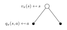
We can discover that the value of a state can be denoted as

$V^\pi(s)=\sum_{a\in A}\pi(a|s)Q_\pi(s,a)$.

In a similar way, Figure 7 shows what states that an action can lead to.

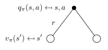
We can also find that

$Q_\pi(s,a)=R(s,a)+\gamma\sum_{s’\in S} P(s’|s,a)V^\pi(s’)$.

On the right-hand side, the first part is the value of the state $s$, the second part is the sum of the product of the value of new state $s’$ and the probability of getting into that new state.

If we combine the two Bellman equation with each other, we can get

$V^\pi(s)=\sum_{a\in A}\pi(a|s)[R(s,a)+\gamma\sum_{s’\in S}P(s’|s,a)V^\pi(s’)]$

​ $=R(s’,\pi(s’))+\gamma\sum_{s’\in S}P(s’|s,\pi(s)) V^\pi(s’)$,

and

$Q_\pi(s,a)=R(s,a)+\gamma\sum_{s’\in S} P(s’|s,a)\sum_{a\in A}\pi(a’|s’)Q_\pi(s’,a’)$.

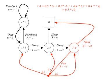
The example in Figure 8 shows that how to calculate the state value of the state represented by the red circle. Notice that actions $Study$ and $Pub$ have the same probabilities $\pi(a|s)$ to be executed, which means they are all $0.5$.

Optimality value function (Bellman optimality equation)

• Optimality state value function $V^*(s)=\tt max\mit V^\pi(s)$ indicates a state value function generated by a policy that makes the value of state $s$ the biggest.
• Optimality state-action value function $Q^*(s,a)=\tt max\mit Q_\pi(s,a)$ indicates a state-action value function generated by a policy that makes the value of the state-action $(s,a)$ the biggest.

Optimality value function determines the best performance of a MDP. When we know the optimality value function, we know the best policy and the best value of every state, and the MDP problem is solved. Solving an optimality value function require us to solve the best policy at first.

Find the best policy

The best policy is defined precisely as optimal policy $\pi^ *$ , which means for every policy $\pi$, for all time steps, and for all states $s\in S$ , there is $V_t^{\pi^ *}(s)\geq V_t^\pi(s)$.

For an infinite horizon MDP, existence of an optimal policy also implies the existence of a stationary optimal policy. Although there is an infinite horizon, we still just need to search finite policies, which equals $|A|^{|S|}$. Moreover, the optimal policy might not be unique.

We can compute the optimal policy by

$\pi^*(s)=\tt argmax\mit V^\pi(s)$,

Which means finding the arguments ($V(s),\pi(s)$) that produce the biggest value function.

If an optimal policy exists then its value function must be a fixed point of the operator $B^*$.

Bellman optimality backup operator

Bellman optimality backup operator is written as $B^*$ with a value function behind it

$B^*V(s)=\tt max_a \mit R(s,a)+\gamma\sum_{s’\in S}P(s’|s,a)V(s’)$.

If $\gamma<1$, $B^*$ is a strict contraction and has a unique fixed point. This means

$B^*V(s)\geq V^\pi(s)$.

Bellman operator return to a new value function and it will improve the value if possible. Sometimes we will use $BV$ to replace Bellman operator and substitute the $V$ on right-hand side of the equation.

Next I’ll briefly introduce some algorithms to compute the optimal value function and an optimal policy.

Policy search

This algorithm is very simple but acquires a great number of computing resources. What it do is just trying all the possible policies and find out the biggest value function, return a value function and a policy.

Policy iteration

The algorithm of policy iteration is shown below:

while True do

​ $V^\pi$ = Policy evaluation $(M,\pi,\epsilon)$ ($\pi$ is initialized randomly here)

​ $\pi^*$ = Policy improvement $(M,V^\pi)$

if $\pi^*(s)=\pi(s)$ then

​ break

else

​ $\pi$ = $\pi^*$

$V^*$ = $V^\pi$ .

Policy evaluation is about how to compute the value of a policy. As for policy improvement, we need to compute

$Q_{\pi i}(s,a)=R(s,a)+\gamma\sum_{s’\in S} P(s’|s,a)V^{\pi i}(s’)$

for all the $a$ and $s$ and then take the max

return $\pi_{i+1}=\tt argmax\mit Q_{\pi i}(s,a)$.

Notice that there is a relationship

$\tt max\mit Q_{\pi i}(s,a)\geq Q_{\pi i}(s,\pi_i(s))$.

This means the agent may adopt the new policy and take better actions (greater) or it just take actions following the former policy (equal). After the improvement the new policy will be monotonically better than the old policy. At the same time, once the policy converge it will never change again.

Value iteration

The algorithm of value iteration is shown below:

$V’(s)=0, V(s)=\infty$, for all $s\in S$

while $||V-V’||_\infty>\epsilon$ do

​ $V=V’$

​ $V’(s)=\tt max\mit_aR(s,a)+\gamma\sum_{s’\in S}P(s’|s,a)V’(s)$, for all states $s\in S$

$V^*=V$, for all $s\in S$

$\pi^ *=\tt argmax_{a\in A}\mit R(s,a)+\gamma\sum_{s’\in S}P(s’|s,a)V^ *(s’),\ \forall s\in S$ .

The idea is to run fixed point iterations to find the fixed point $V^* $ of $B^ *$.